[Introduction to Algorithm] Linear Time Sorting

Although all comparision sorting algorithm requires at least \(\Omega(n\lg n)\) comparisons, in certain conditions, we are able to sort an array in \(O(n)\) complexity.

Comparison Sort

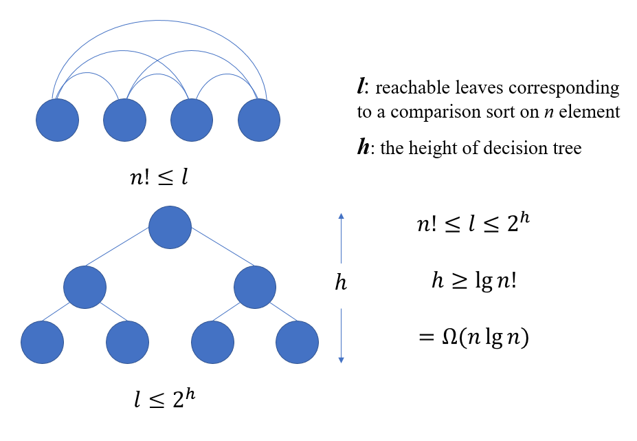
Any comparison sort algorithm requires \(\Omega(n\lg n)\) comparisons in the worst case.

Proof:

1538536652121

Counting Sort

1538538894641

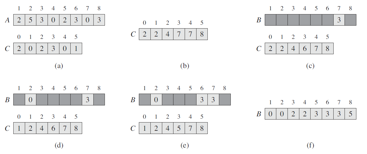
def COUNTING_SORT(A, B, k):
    # A[] is the input array
    # B[] is the array with same length
    # k is the max value in the array
    C = []
    for i in range(0, k):
        C[i] = 0
    for j in range(1, k):
        C[A[j]] += 1
    // C[i] now comtains the number of elements equal to i   (a)
    for i in range(1, k):
        C[i] = C[i] + C[i-1]
    // C[i] now contains the number of elements less than or equal to i   (b)
    for j in range(A.length, 1):
        B[C[A[j]]] = A[j]
        C[A[j]] -= 1

Radix Sort

1538622405267

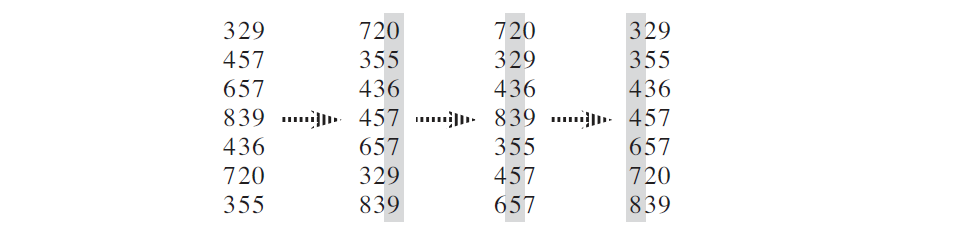
def RADIX_SORT(A, d):
    for i = 1 to d:
        use Count_Sort to sort array A on digit i

\(\Theta(d(n+k))\), while d is numbers digits, k is each digits take on up to k possible values.

Bucket Sort

1538804822506

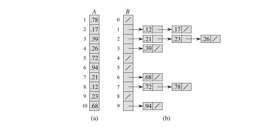
Implementation

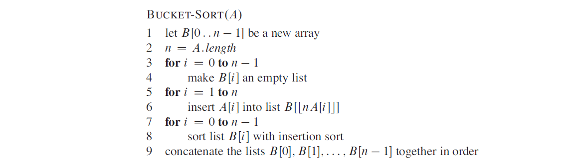
1538805969015

Analysis

The running time of bucket sort: \[ T(n) = \Theta(n) + \sum_{i=0}^{n-1}O(n_{i}^2) \]

Since we are analyze the average case, we compute the expectation:

\[ E[T(n)]=E[\Theta(n)+\sum_{i=0}^{n-1}O(n_{i}^2)] \]

\[ =\Theta(n)+\sum_{i=0}^{n-1}E[O(n_{i}^2)] \]

\[ =\Theta(n)+\sum_{i=0}^{n-1}O[E(n_{i}^2)] \]

We claim that

\[ E(n_{i}^2)=2-1/n \tag{1} \] (Proved later)

Then

\[ E[T(n)] = \Theta(n) + \sum_{i=0}^{n-1}O(2)=\Theta(n) \]

Now we prove (1):

\[ We \ define\ indicator\ random\ variables \]

\[ X_{ij} =I\{A[ j] \ falls\ in\ bucket\ i\} \]

Thus,

\[ n_i=\sum_{j=0}^{n}X_{ij} \]

Then,

\[ E[n_i^2]=E[(\sum_{j=0}^{n}X_{ij})^2] \]

\[ \ \ \ \ \ \ \\ \ =E[\sum_{j=0}^{n}X_{ij}^2+\sum_{j=1}^{n}\sum_{k=1 while\ k\neq j}^{n}X_{ij}X_{ik}] \]

\[ \ \ \ \ \ \ \\ \ =\sum_{j=0}^{n}E[X_{ij}^2]+\sum_{j=1}^{n}\sum_{k=1 while\ k\neq j}^{n}E[X_{ij}X_{ik}]\tag{2} \]

Indicator random variable \(X_{ij}\) is 1 with probability 1/n and 0 otherwise.

Then,

\[ E[X_{ij}^2] = 1^2\cdot\frac{1}{n} + 0^2\cdot(1-\frac{1}{n}) \]

\[ =\frac{1}{n} \]

When \(k\neq j\), the variables \(X_{ij}\) and \(X_{ik}\) are independent.

Then,

\[ E[X_{ij}X_{ik}] = \frac{1}{n}\cdot\frac{1}{n} = \frac{1}{n^2} \]

Therefore, (2)

\[ E[n_i^2] =\sum_{j=1}^n\frac{1}{n} +\sum_{j=1}^{n}\sum_{k=1 while\ k\neq j}^{n}\frac{1}{n^2} \]

\[ =n\cdot\frac{1}{n}+n(n-1)\cdot\frac{1}{n^2} \]

\[ =2-\frac{1}{n} \]